MISMIP3d
The ice2sea MISMIP3d intercomparison is a two-horizontal-dimensional extension of the flowline case described above. As before, in MISMIP3d the grounding line position and its reversibility under changes of physical parameters is analyzed. Instead of changing the ice softness, however, the spatial distribution and magnitude of basal friction is adjusted between experiments. The applied basal friction perturbation of the basal friction is a localized gaussian “bump” and thus a curved grounding line is obtained. In contrast to the flowline experiments, no (semi-)analytical solutions are available to compare to the numerical results.
A full description of the MISMIP3d experiments can be found at
and the results are published in [126].
A complete set of MISMIP3d experiments consists of three runs: Firstly, a flowline
solution on a linearly-sloped bed, similar to the flowline MISMIP experiments of the
previous section, is run into a steady state (“standard experiment Stnd”). Then the
localized sliding perturbation is applied (“perturbation experiment”) causing the
grounding line to shift and lose symmetry. Two different amplitudes of the perturbation
are considered (”P10” and “P75”). Finally, beginning from the final state of the
perturbation experiment, the sliding perturbation is removed and the system is run again
into steady state (“reversibility experiment”). The resulting geometry, in particular the
grounding line position, is expected to be close to that of the standard experiment.
Expecting such reversibility assumes that a particular stationary ice geometry only
depends on its physical parameters and boundary conditions and not on how it is
dynamically reached.
For these experiments in PISM, a Python script generates a shell script which has the
commands and options for running a MISMIP3d experiment. The python script is
createscript.py in the folder examples/mismip/mismip3d/. Run
./createscript.py -h
to see a usage message. A README.md gives a tutorial on how to use createscript.py
and do the runs themselves.
For the flowline Stnd experiment, as in the MISMIP case, a computational domain with
three grid points in the direction orthogonal to the ice flow (arbitrarily chosen as
y-direction) is chosen by createscript.py. For the perturbation and reversibility
experiments a domain is defined which is symmetric along the ice-divide (mirror symmetry)
and along the center line of the ice flow, while the side boundaries are periodic, which
corresponds to a free-slip condition for the flow in x-direction. Though this choice of
the symmetric computational domain increases computational cost, it allows us to use
standard PISM without fixing certain boundary conditions in the code. (That is, it avoids
the issues addressed in the regional mode of PISM; see section Example: A regional model of the Jakobshavn outlet glacier in Greenland.)
PISM participated in the MISMIP3d intercomparison project [126] using version pism0.5, and the exact results can be reproduced using that version. PISM’s results, and the role of resolution and the new subgrid grounding line interpolation scheme are discussed in [101].
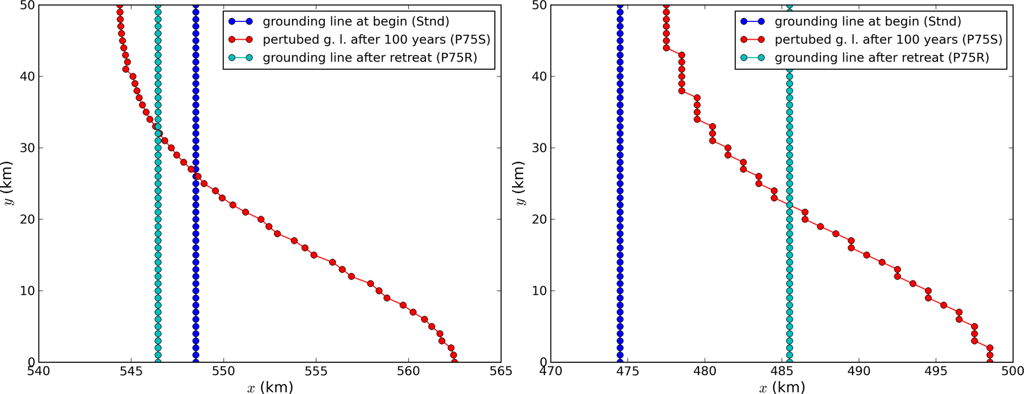
We observed a considerable improvement of the results with respect to the absolute
grounding line positions compared to other models (e.g. the FE reference model Elmer/Ice)
and to the reversibility when applying the subgrid grounding line interpolation method;
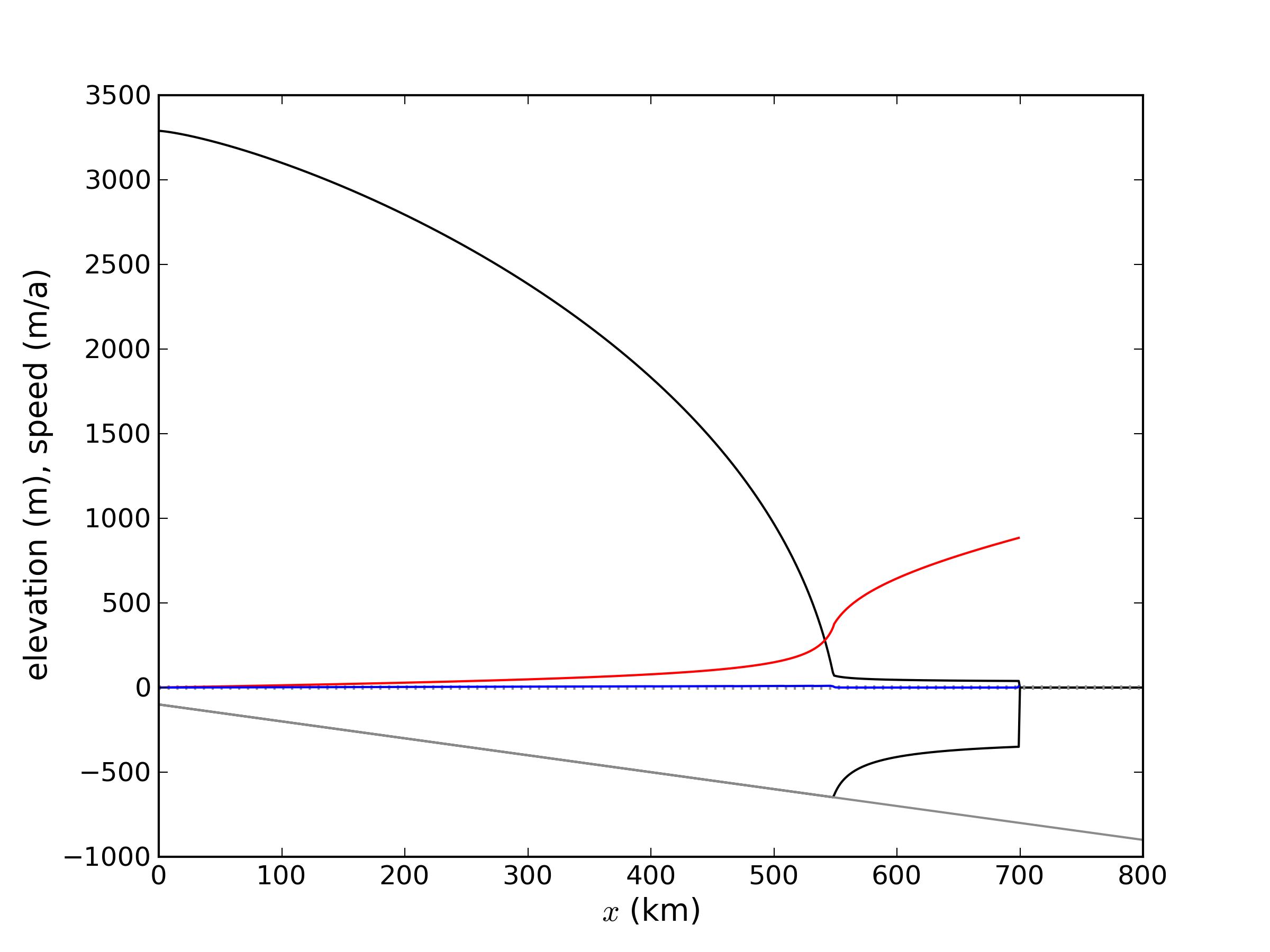
see Fig. 26. Furthermore, we observed that only using SSA yields almost
the same results as the full hybrid SIA+SSA computation for the MISMIP3D (and also the
MISMIP) experiments, but, when not applying the SIA computation, after a considerably
shorter computation time (about 10 times shorter). We explain the small and almost
negligible SIA velocities for the MISMIP(3D) experiments with the comparably small ice
surface gradients in the MISMIP3d ice geometries. See Fig. 27 for a
comparison of SSA and SIA velocities in the MISMIP3D geometry. Note that both Figures
Fig. 26 and Fig. 27 were generated with resolution of

Fig. 26 Comparison between the grounding lines of the higher-amplitude (”P75”) MISMIP3d
experiments performed with PISM when using the subgrid grounding line interpolation
method (left) or not using it (right). In both cases the SIA+SSA hybrid is used.

Fig. 27 The SIA velocities are negligible in the MISMIP3d standard experiment (”Stnd”). The
steady state ice geometry is plotted (black) together with the computed SSA velocity
(red) and SIA velocity (blue). The SIA velocity reaches its maximum value of about
| Previous | Up | Next |
