An ice dynamics parameter study¶

The readers of this manual should not assume the PISM authors know all the correct parameters for describing ice flow. While PISM must have default values of all parameters, to help users get started,[1] it has more than five hundred user-configurable parameters. The goal in this manual is to help the reader adjust them to their desired values. While “correct” values may never be known, or may not exist, examining the behavior of the model as it depends on parameters is both a nontrivial and an essential task.

For some parameters used by PISM, changing their values within their ranges of experimental uncertainty is unlikely to affect model results in any important manner (e.g. constants.sea_water.density). For others, however, for instance for the exponent in the basal sliding law, changing the value is highly-significant to model results, as we’ll see in this subsection. This is also a parameter which is very uncertain given current glaciological understanding [34].

To illustrate a parameter study in this Manual we restrict consideration to just two important parameters for ice dynamics,

$q =$ basal_resistance.pseudo_plastic.q: exponent used in the sliding law which relates basal sliding velocity to basal shear stress in the SSA stress balance; see subsection Controlling basal strength for more on this parameter, and
$e =$ stress_balance.sia.enhancement_factor: values larger than one give flow “enhancement” by making the ice deform more easily in shear than is determined by the standard flow law [35], [36]; applied only in the SIA stress balance; see section Ice rheology for more on this parameter.

By varying these parameters over full intervals of values, say $0.1 \leq q \leq 1.0$ and $1 \leq e \leq 6$ , we could explore a two-dimensional parameter space. But of course each $(q, e)$ pair needs a full computation, so we can only sample this two-dimensional space. Furthermore we must specify a concrete run for each parameter pair. In this case we choose to run for 1000 model years, in every case initializing from the stored state g10km_gridseq.nc generated in the previous section Grid sequencing.

The next script, which is param.sh in examples/std-greenland/, gets values $q \in {0.1, 0.5, 1.0}$ and $e \in {1, 3, 6}$ in a double for-loop. It generates a run-script for each $(q, e)$ pair. For each parameter setting it calls spinup.sh, with the environment variable PISM_DO=echo so that spinup.sh simply outputs the run command. This run command is then redirected into an appropriately-named .sh script file:

#!/bin/bash

NN=8
DURATION=1000
START=g10km_gridseq.nc
for PPQ in 0.1 0.5 1.0 ; do
  for SIAE in 1 3 6 ; do
     export PISM_DO=echo REGRIDFILE=$START PARAM_PPQ=$PPQ PARAM_SIAE=$SIAE
     ./spinup.sh $NN const $DURATION 10 hybrid p10km_${PPQ}_${SIAE}.nc &> p10km_${PPQ}_${SIAE}.sh
  done
done

Notice that, because the stored state g10km_gridseq.nc used $q = 0.5$ and $e = 3$ , one of these runs simply continues with no change in the physics.

To set up and run the parameter study, without making a mess from all the generated files, do:

cd examples/std-greenland/           # g10km_gridseq.nc should be in this directory
mkdir paramstudy
cd paramstudy
ln -s ../g10km_gridseq.nc .            # these four lines make links to ...
ln -s ../pism_Greenland_5km_v1.1.nc .  #
ln -s ../spinup.sh .                   #
ln -s ../param.sh .                    # ... existing files in examples/std-greenland/
./param.sh

The result of the last command is to generate nine run scripts,

p10km_0.1_1.sh  p10km_0.1_3.sh  p10km_0.1_6.sh
p10km_0.5_1.sh  p10km_0.5_3.sh  p10km_0.5_6.sh
p10km_1.0_1.sh  p10km_1.0_3.sh  p10km_1.0_6.sh

The reader should inspect a few of these scripts. They are all very similar, of course, but, for instance, the p10km_0.1_1.sh script uses options -pseudo_plastic_q 0.1 and -sia_e 1.

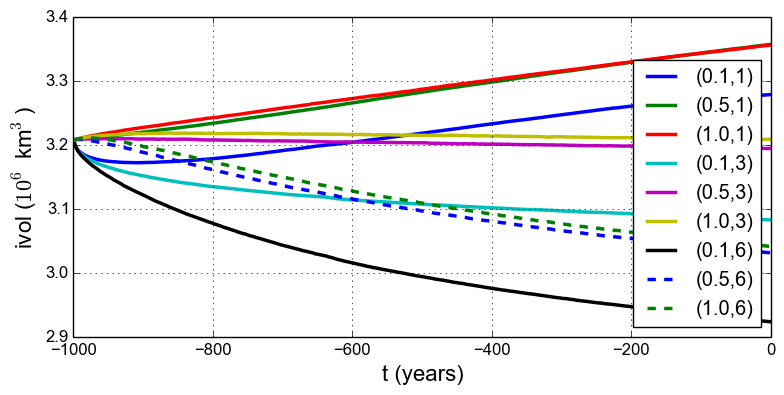
../../_images/ivol-param.png — Fig. 12 Time series of ice volume `ice_volume_glacierized` from nine runs in our parameter study example, with parameter choices $(q, e)$ given.¶

We have not yet run PISM, but only asked one script to create nine others. We now have the option of running them sequentially or in parallel. Each script itself does a parallel run, over the NN=8 processes specified by param.sh when generating the run scripts. If you have $8 \times 9 = 72$ cores available then you can do these runs fully in parallel (this is runparallel.sh in examples/std-greenland/):

#!/bin/bash

for scriptname in $(ls p10km*sh) ; do
  echo ; echo "starting ${scriptname} ..."
  bash $scriptname &> out.$scriptname &  # start immediately in background
done

Otherwise you should do them in sequence (this is runsequential.sh in examples/std-greenland/):

#!/bin/bash

for scriptname in $(ls p10km*sh) ; do
  echo ; echo "starting ${scriptname} ..."
  bash $scriptname                       # will wait for completion
done

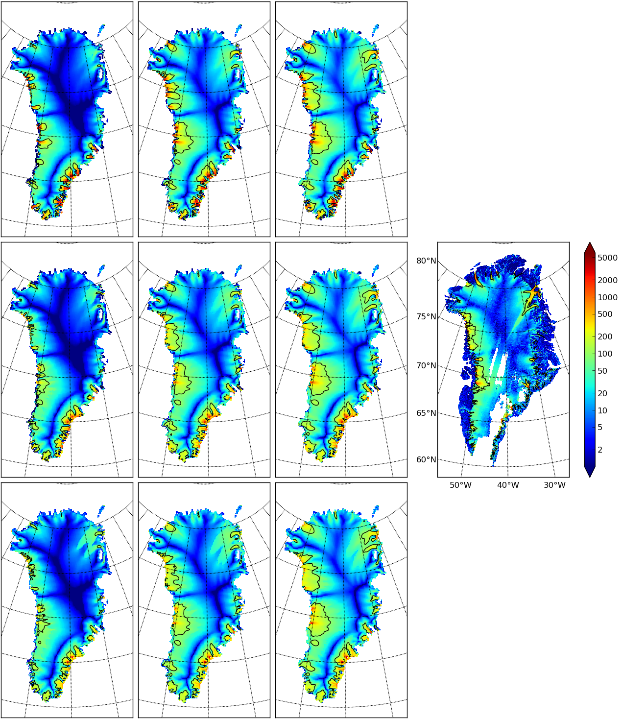
On the same old 2020-era 8 core laptop, runsequential.sh took a total of about 4 hours to complete the whole parameter study. The runs with $q = 0.1$ (the more “plastic” end of the basal sliding spectrum) took up to four times longer than the $q = 0.5$ and $q = 1.0$ runs. Roughly speaking, values of $q$ which are close to zero imply a subglacial till model with a true yield stress, and the result is that even small changes in overall ice sheet state (geometry, energy, …) will cause some location to exceed its yield stress and suddenly change flow regime. This will shorten the time steps. By contrast, the $e$ value is much less significant in determining run times.

../../_images/p10km-comparison.png — Fig. 13 Surface speed `velsurf_mag` from a 10 km grid parameter study. Right-most sub-figure is observed data from `Greenland_5km_v1.1.nc`. Top row: $q = 0.1$ and $e = 1, 3, 6$ (left-to-right). Middle row: $q = 0.5$ . Bottom row: $q = 1.0$ . All subfigures have common color scale (velocity m/year), as shown in the right-most figure, with 100 m/year contour shown in all cases (solid black).¶

On a supercomputer, the runparallel.sh script generally should be modified to submit jobs to the scheduler. See example scripts advanced/paramspawn.sh and advanced/paramsubmit.sh for a parameter study that does this. (But see your system administrator if you don’t know what a “job scheduler” is!) Of course, if you have a supercomputer then you can redo this parameter study using a finer grid.

Results from these runs are seen in Fig. 12 and Fig. 13. In the former we see that the $(0.5, 3)$ run simply continues the previous initialization run. In some other graphs we see abrupt initial changes, caused by abrupt parameter change, e.g. when the basal sliding becomes much more plastic ( $q = 0.1$ ). In all cases with $e = 1$ the flow slows and the sheet grows in volume as discharge decreases, while in all cases with $e = 6$ the flow accelerates and the sheet shrinks in volume as discharge increases.

In Fig. 13 we can compare the modeled surface speed to observations. Roughly speaking, the ice softness parameter $e$ has effects seen most-clearly by comparing the interior of the ice sheet; scan left-to-right for the $e = 1, 3, 6$ subfigures. The basal sliding exponent $q$ has effects seen most-clearly by comparing flow along the very steep margin, especially in the southern half of the ice sheet; scan top-to-bottom for $q = 0.1, 0.5, 1.0$ , going from nearly-plastic at top to linear at bottom.

From such figures we can make an informal assessment and comparison of the results, but objective assessment is important. Example objective functionals include:

compute the integral of the square (or other power) of the difference between the model and observed surface velocity [2], or
compute the model-observed differences between the histogram of the number of cells with a given surface speed [37].

Note that these functionals are measuring the effects of changing a small number of parameters, namely two parameters in the current study. So-called “inversion” might use the same objective functionals but with a much larger parameter space. Inversion is therefore capable of achieving much smaller objective measures [27], [25], [24], though at the cost of less understanding, perhaps, of the meaning of the optimal parameter values.

Footnotes