Second run: a better ice-dynamics model

It is widely-understood that ice sheets slide on their bases, especially when liquid water is present at the base (see [13], [14], among others). An important aspect of modeling such sliding is the inclusion of membrane or “longitudinal” stresses into the stress balance [10]. The basic stress balance in PISM which involves membrane stresses is the Shallow Shelf Approximation (SSA) [15]. The stress balance used in the previous section was, by contrast, the (thermomechanically-coupled) non-sliding, non-membrane-stress Shallow Ice Approximation (SIA) [16], [12]. The preferred ice dynamics model within PISM, that allows both sliding balanced by membrane stresses and shear flow as described by the SIA, is the SIA+SSA “hybrid” model [10], [17]. For more on stress balance theories see section Ice dynamics, the PISM view of this Manual.

The practical issue with models of sliding is that a distinctly-uncertain parameter space must be introduced. This especially involves parameters controlling the amount and pressure of subglacial water (see [2], [18], [19], [20], among others). In this regard, PISM uses the concept of a saturated and pressurized subglacial till with a modeled distribution of yield stress [10], [21]. The yield stress arises from the PISM model of the production of subglacial water, which is itself computed through the conservation of energy model [22]. We use such models in the rest of this Getting Started section.

While the spinup.sh script has default sliding-related parameters, for demonstration purposes we change one parameter. We replace the default power $q=0.25$ in the sliding law (the equation which relates both the subglacial sliding velocity and the till yield stress to the basal shear stress which appears in the SSA stress balance) by a less “plastic” and more “linear” choice $q=0.5$. See section Controlling basal strength for more on sliding laws. To see the run we propose, do

PISM_DO=echo PARAM_PPQ=0.5 ./spinup.sh 8 const 10000 20 hybrid g20km_10ka_hy.nc

Now remove “PISM_DO=echo” and redirect the text output into a file to start the run:

PARAM_PPQ=0.5 ./spinup.sh 8 const 10000 20 hybrid g20km_10ka_hy.nc &> out.g20km_10ka_hy &

This run should take 10 minutes or less.[1]

When this run is finished it produces g20km_10ka_hy.nc. As before do

ncdump -h g20km_10ka_hy.nc | grep -E "run_stats:.+hour"

to see performance results for your machine.

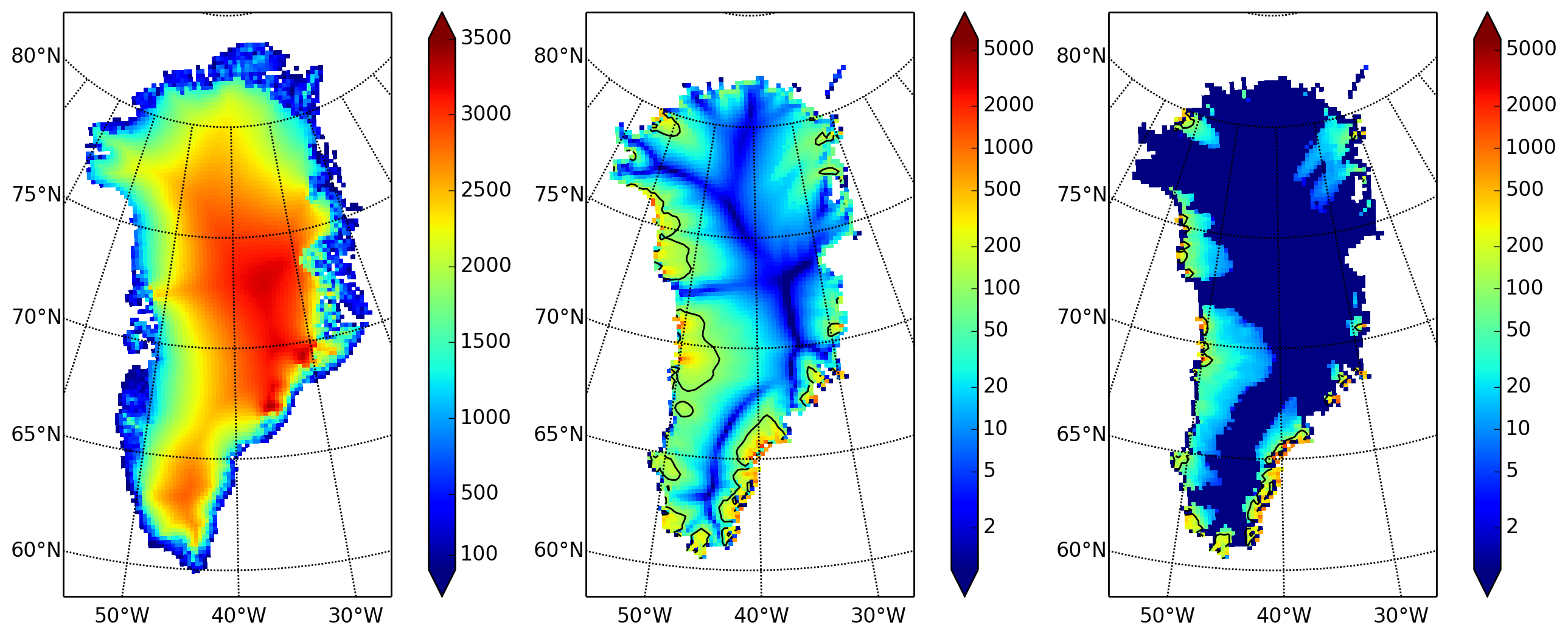
The results of this run are shown in Fig. 4. We show the basal sliding speed field velbase_mag in this Figure, where Fig. 3 had the mask, but the reader can check that velbase_mag is zero in the nonsliding SIA-only result g20km_10ka.nc.

Fig. 4 Fields from output file g20km_10ka_hy.nc.

Left:

usurf, the ice sheet surface elevation in meters.

Middle:

velsurf_mag, the surface speed in m/year, including the 100 m/year contour (solid black).

Right:

the sliding speed velbase_mag, shown the same way as velsurf_mag.

The hybrid model includes sliding, and it is important to evaluate that aspect of the output. However, though it is critical to the response of the ice to changes in climate, basal sliding velocity is essentially unobservable in real ice sheets. On the other hand, because of relatively-recent advances in radar and image technology and processing [23], the surface velocity of an ice sheet can be measured.

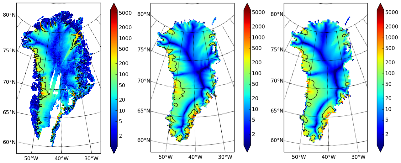
So, how good is our model result velsurf_mag? Fig. 5 compares the radar-observed surfvelmag field in the downloaded SeaRISE-Greenland data file Greenland_5km_v1.1.nc with the just-computed PISM result (20 km) and results from the next step in the tutorial (10 km). The reader might agree with these broad qualitative judgements:

• the model results and the observed surface velocity look similar, and

• slow near-divide flow is generally in the right areas and of generally the right magnitude, but

• the observed Northeast Greenland ice stream is more distinct than in the model.

Fig. 5 Comparing observed and modeled surface speed.

All figures have a common scale (m/year), with 100 m/year contour shown (solid black).

Left:

surfvelmag, the observed values from SeaRISE data file Greenland_5km_v1.1.nc.

Middle:

velsurf_mag from g10km_10ka_hy.nc (will be run in next step of tutorial).

Right:

velsurf_mag from g20km_10ka_hy.nc.

We can compare these PISM results to other observed-vs-model comparisons of surface velocity maps, for example Figure 1 in [24] and Figure 8 in [25]. Only ice-sheet-wide parameters and models were used here in PISM, that is, each location in the ice sheet was modeled by the same physics. By comparison, those published comparisons involved tuning a large number of spatially-variable subglacial parameters to values which would yield close match to observations of the surface velocity. Such tuning techniques, called “inversion” or “assimilation” of the surface velocity data, are also possible in PISM,[2] but the advantage of having few parameters in a model is well-known: the results reflect the underlying model, not the flexibility of many parameters.

We have only tried two of the many models possible in PISM, and we are free to identify and adjust important parameters. The first parameter change we consider, in the next subsection, is one of the most important: grid resolution.

Footnotes

[1]

Regarding the relative speeds of the runs that produce g20km_10ka.nc and g20km_10ka_hy.nc, note that the computation of the SSA stress balance is substantially more expensive than the SIA in a per-step sense. However, the SSA stress balance in combination with the mass continuity equation causes the maximum diffusivity in the ice sheet to be substantially lower during the run. Because the maximum diffusivity controls the time-step in the PISM adaptive time-stepping scheme [16], the number of time steps is reduced in the hybrid run. To see this contrast use ncview ts_g20km_10ka*nc to view variables max_diffusivity and dt.

[2]

See [26] (inversion of DEMs for basal topography) and [27] (inversion surface velocities for basal shear stress) for PISM-based inversion methods and analysis.

---

Previous

Up

Next